Six structured lessons connect process-control principles to simulated practice. Start by reading the evidence, work through the calculation, test the idea in a Lab, then explain what would make the decision unsafe. Each lesson includes an answer you can reveal after attempting the learning check.
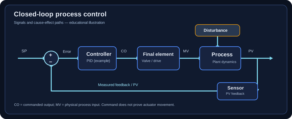
Original explanatory schematic: commanded output is not physical valve movement. Trace the measured feedback path before deciding which variable has changed.
How to study the series
Predict: make a written prediction before viewing the example.
Calculate: recreate the worked result and record units and assumptions.
Simulate: compare your reasoning with the synthetic Lab scenario and save evidence.
Defend: explain a competing diagnosis, an uncertainty and a stop condition.
Retrieve: repeat the question two days later and after one or two weeks.
These lessons are supplemental education, not an assessed result, accredited credential or authorization to change live process equipment.
Lesson 01 · Foundation · 15–20 min
Read the loop before touching the tuning
Recognize the process variable (PV), setpoint (SP), controller output (CO), manipulated variable (MV) and final control element. Explain the control objective in ordinary plant language.
What you need to know
Identify the sensor, controller, output path, final element and process response on a basic P&ID. CO is often a percentage command; MV is the physical quantity changed, such as valve flow.
Distinguish a setpoint move from an output step. They are not interchangeable for identifying open-loop process dynamics.
Check units, engineering ranges, sample interval, operating mode, controller action and whether output limits or permissives are active.
Ask which process constraints matter: product quality, pressure, level limits, environmental consequences and valve travel.
Worked example
A cooling-water flow loop
A flow transmitter reads 72 m³/h while SP is 80 m³/h. The controller output is 44% to a modulating valve. The process engineer observes that increasing output opens the valve and raises flow.
PV = 72 m³/h; SP = 80 m³/h; the indicated error SP − PV is +8 m³/h. Error sign conventions vary by controller.
CO = 44% is a command, not the measured water flow. The manipulated flow depends on actual valve position, supply pressure and equipment conditions.
Document whether valve action is air-to-open or air-to-close and the controller action convention. Do not infer a safe output direction from the error sign alone.
Interpretation: Before selecting a PID gain, the learner can draw the causal chain from controller output to valve to flow transmitter and explain every displayed quantity.
Stop / escalate decision
If controller action, valve fail position or output authority is uncertain, stop. Request the loop sheet, instrument data, operating procedure and authorized review.
Common misconception
Treating a changing valve command as proof that the valve moved. Stiction, positioner faults or limits can break that assumption.
Try it in a Lab
Open a clean introductory flow case. Label PV and output, then predict the direction of the measured response before inspecting the trend.
Practice a flow loop →Check your understanding: What is the difference between CO and MV?
CO is the controller command; MV is the physical process input it influences. They may differ when actuators, limits or disturbances intervene.
Use a bounded synthetic output step to estimate first-order-plus-dead-time (FOPDT) gain, lag and delay without treating poor evidence as a valid model.
What you need to know
For a settled step response, process gain Kp is approximately (final PV − initial PV) divided by (final CO − initial CO). Retain the sign and engineering units.
Dead time θ is the interval after the step before a meaningful response appears; time constant τ is measured from the response onset to roughly 63.2% of the total first-order change.
Identify pre-step stability, adequate excitation, sufficiently long observation, signal quality and disturbances before interpreting any fit.
A plausible numeric fit does not make a poorly designed test acceptable. Noise, drift, interacting loops, oscillation and no actual output step can require review or refusal.
Worked example
Calculate Kp, θ and τ
A synthetic flow test starts at PV = 50 and CO = 40%. At t = 10 s, CO steps to 45%. The settled PV is 57; a meaningful response starts at approximately t = 11 s and reaches PV ≈ 54.42 at t ≈ 17 s.
Kp ≈ 7 / 5 = +1.4 PV units per CO percentage point.
θ ≈ 11 − 10 = 1 s. The 63.2% response level is 50 + 0.632 × 7 ≈ 54.42.
τ ≈ 17 − 11 = 6 s, measured after dead time. State uncertainty due to sample spacing and noise.
Interpretation: A defensible preliminary model is Kp ≈ 1.4, τ ≈ 6 s, θ ≈ 1 s, conditional on the stated data quality and first-order approximation.
Stop / escalate decision
Refuse an identification if the actuator never actually steps or if another disturbance dominates the response. Report what evidence is missing rather than fabricating a model.
Common misconception
Measuring τ from the command step instead of the beginning of the process response, thereby mixing delay into lag.
Try it in a Lab
Use a clean flow case, export CSV, estimate the three parameters by hand, and compare with the owned synthetic ground truth and LoopIQ Identify.
Compare model evidence →Check your understanding: Can a good-looking fit from a tiny noisy step automatically be accepted?
No. Excitation and signal-to-noise limits must be documented. A numerical fit without credible test evidence may require review or refusal.
Explain why tuning rules differ, how a response-speed target changes robustness, and why simulated results must be checked against operating limits.
What you need to know
Know the controller algorithm form and units before transferring tuning parameters. Parallel, ideal and series/interacting forms are not numerically interchangeable.
The IMC/SIMC family uses a desired closed-loop time scale, often denoted λ, to trade speed for tolerance of model error and disturbances.
Do not use a tuning formula blindly for integrating, unstable, strongly nonlinear or interacting processes; select a compatible model and review safety constraints.
Evaluate SP tracking, disturbance rejection, overshoot, output movement, saturation and response to plant/model mismatch. A fast response alone is not a quality verdict.
Worked example
Compare a conservative and aggressive PI target
For a synthetic stable FOPDT model Kp = 2, τ = 20 s and θ = 4 s, consider the common IMC-style PI approximation Kc = τ/[Kp(λ + θ)] with Ti = min(τ, 4(λ + θ)) for the simplified stable-FOPDT SIMC PI case. The formula is illustrative; controller conventions and method applicability must be checked.
For λ = 20 s: Kc ≈ 20/[2(20 + 4)] ≈ 0.417; Ti = min(20, 96) = 20 s.
For λ = 8 s: Kc ≈ 20/[2(8 + 4)] ≈ 0.833; Ti = min(20, 48) = 20 s.
The shorter λ produces roughly twice the proportional gain in this example. That may speed nominal response but increases sensitivity to delay error and valve activity.
Run both settings in the simulator against disturbance, noise, output limits and modest parameter mismatch; compare trends and note that no live-controller settings are authorized.
Interpretation: The more aggressive numeric setting is not automatically preferable. Choose based on the actual performance requirement and verified robustness margin.
Stop / escalate decision
When model accuracy or actuator health is doubtful, use a conservative study case or escalate; do not optimize around an unverified plant model.
Common misconception
Copying Kc and Ti into a controller configured for a different action or algorithm form.
Try it in a Lab
Compare two tuning choices on the same synthetic loop. Record overshoot, settling behavior, command movement and what happens under mismatch.
It can reduce sensitivity to plant/model mismatch, dead-time uncertainty and excessive actuator movement, though each trade-off requires simulation and engineering review.
Diagnose valve and measurement faults before tuning
Separate a controller-tuning problem from instrument faults, valve nonlinearities and process disturbances.
What you need to know
Valve stiction can produce repeated output ramps followed by abrupt PV changes. Hysteresis and deadband can prevent small output commands from producing proportional movement.
Compare controller output, position feedback (when reliable), independent measurements, instrument alarms and process constraints. Correlation alone is not root-cause proof.
An oscillating trend may be caused by an overly aggressive controller, interacting loops, valve faults or cyclic disturbances. The remedy depends on the cause.
Record competing hypotheses and choose the least disruptive safe test that discriminates between them.
Worked example
Why changing Kc may not fix the loop
A simulated level loop shows CO increasing gradually from 42% to 51% while the PV stays nearly constant, followed by a sudden PV jump. This repeats with similar thresholds.
The delayed, abrupt PV movements after accumulated command are more consistent with actuator nonlinearity than a simple low-gain first-order response.
Inspect simulated position feedback and alternate sensor evidence. If physical actuator behavior is unverified, mark the diagnosis provisional.
Recommend inspection or an approved positioner/valve assessment; do not claim that increasing gain repairs a sticking valve.
Interpretation: A strong diagnostic answer explains the evidence, alternate causes and the next safe discriminating test—not just the preferred tuning value.
Stop / escalate decision
Stop if a valve is at a limit, the process is near a trip threshold, or movement could affect a safety function. Follow the site permit and management-of-change process.
Common misconception
Using tuning changes to conceal an instrument or mechanical defect that later reappears as a safety or quality problem.
Try it in a Lab
Complete the valve nonlinearity and field-judgment exercises. State at least two competing diagnoses and what could falsify each.
Practice fault diagnosis →Check your understanding: Does repeating oscillation prove that the PID settings are wrong?
No. Stiction, deadband, disturbances and interactions can produce similar symptoms. A discriminating diagnosis is needed first.
Make decisions that remain defensible when a synthetic model differs from the actual process.
What you need to know
Use sensitivity concepts to explain why nominally fast loops can become fragile under dead-time, gain or lag mismatch.
Maximum sensitivity (Ms), phase margin and gain margin are robustness indicators, not universal promises of stability under all nonlinearities or operating conditions.
Challenge a proposed tuning with gain, lag and delay variations and with output saturation, sensor noise and disturbances.
Document acceptance criteria before testing: overshoot, settling range, output travel, constraints and stop conditions.
Worked example
A delay-mismatch review
A design assumes θ = 3 s but an alternate synthetic test suggests θ = 7 s. A fast tuning set was selected from the original model.
Record the new delay as a material model difference, not a minor rounding error.
Replay both models with identical disturbances and compare output command, overshoot, ringing and any limit approach.
If the changed model violates the predefined acceptance criteria, reject the faster tuning proposal and investigate the source of the delay.
Retain the test parameters and trends so another reviewer can reproduce the decision.
Interpretation: Robustness is an evidence-backed tolerance to uncertainty, not a badge earned by choosing one favorable nominal simulation.
Stop / escalate decision
A simulation can support a proposal but cannot establish field safety, authorization, protection-system adequacy or full plant operating-envelope coverage.
Common misconception
Claiming a single gain-margin or Ms value guarantees safe performance across every operating point.
Try it in a Lab
Run an advanced-control or competency exercise with deliberate model mismatch and prepare a two-column nominal-versus-stressed evidence table.
Understand why cascade, feedforward, ratio, split-range and override structures solve different classes of problems.
What you need to know
Cascade uses a measured secondary variable with a faster inner loop. If the inner loop is not materially faster and reliable, cascade may add complexity without benefit.
Feedforward acts on a measured disturbance before its full PV effect arrives. It needs the correct direction, scaling and timing and usually works alongside feedback.
Ratio control preserves a relationship between two measured streams; validate measurement units, operating limits and what happens at low or zero flow.
Override/select logic protects a constraint by selecting between demands. The selection direction, tracking/anti-windup and loss-of-signal behavior are safety-critical design decisions.
Worked example
Choose between cascade and feedforward
A heater outlet-temperature loop suffers from supply-pressure disturbances. Fuel-flow feedback is available; supply pressure is measured, but the control valve has occasional position feedback faults.
Cascade may improve performance by making a fast, reliable fuel-flow loop the inner controller. First confirm inner-loop dynamics, limits and reliable flow measurement.
Feedforward from measured supply pressure may compensate a predictable disturbance; it needs a calibrated model and feedback trim.
The reported valve feedback fault raises uncertainty. Neither structure should be adopted before assessing actuator behavior and the operating envelope.
Compare the baseline and proposed architectures under the same disturbances and failed-sensor scenarios; document fallback behavior.
Interpretation: Select architecture from measured disturbance paths, secondary-loop capability, constraint ownership and failure response—not from feature sophistication.
Stop / escalate decision
High-consequence process-control architecture changes require independent engineering review, applicable safety studies and employer/site approval. Lab completion grants none of these.
Common misconception
Adding an advanced block without proving failover, bumpless transfer, tracking and operator interpretability.
Try it in a Lab
Choose an L4 advanced-control practical, sketch the block diagram, define fallback behavior and compare baseline against proposed control.
The process-model and illustrative SIMC PI lessons draw on established industrial-control literature. Their calculations are educational examples; no source establishes that these parameters are suitable for a particular installation.
Real-plant work requires current site control narratives, vendor manuals, equipment limits, appropriate engineering reviews and the employer's approved change procedures.